If Word is a tool used to edit documents, with Excel it is in charge of solving math operations on spreadsheets. Usually, for simple math, you just need to use simple functions. However, in some conditional operations, you are forced to use more difficult operations such as the IF function. So, how to use this function, today's article Web888 will share with you about this problem.

The IF function is called the conditional function in Excel. When you use the IF function, it will get you the desired values in Excel columns and rows.

The content of the article consists of 2 parts:

• Introduction to the IF . function
• Illustrated example of the IF . function

1. Introduction to the IF . function

In simple terms, the IF function is an if…then… function. More specifically, it is an operation to test a value against previously given conditions. If it is true, it returns one value, if it is false, it returns another value.

The syntax of the IF function is as follows:

=IF(condition, value 1, value 2)

• If the condition is true then the result will be the value one .
• If the following condition thf the result will be the value two

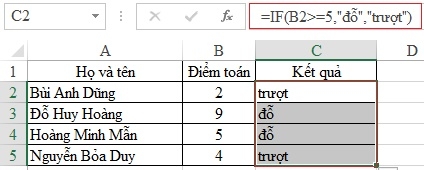
Example: If your math score is greater than or equal to 5 then you pass, otherwise you will fail.

With this post, because you all have the same conditions. Therefore, I just need to calculate the results with Bui Anh Dung first. Then compare that result with the rest. That way, you won't have to enter the function multiple times.

You type the function like this:

=IF(B2>=5,”passed”,”failed”).

Note: When you type literal values, a closing quotation mark is required.

After Anh Dung's results appear, you just need to drag your mouse down to the right corner of the calculated cell and wait for it to appear a "+" sign, then hold the mouse and drag down to the position you need to calculate. Then you release the mouse, all the results appear on the spreadsheet.

2. Example of IF . function

We have the following spreadsheet:

In this worksheet, you need to fulfill the following requirements:

• Calculate the total score of the three subjects of the students
• Calculate the average score of the three subjects of the students
• If a student has a total score of three subjects lower than 15 points, they fail, the rest pass.

We solve each request as follows:

First, to calculate the total score of three subjects, I have instructions for you in the lesson using the SUM function .

Accordingly, we have the following formula:

=SUM(C2:E2)

After outputting the results, you just need to drag the mouse to the bottom right corner of the cell, wait for the "+" sign to appear, then hold the mouse and drag to the position to be calculated and then release the mouse.

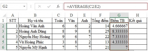
Second, calculate the average of the three subjects for each student.

This is also the problem that I showed you in the post on how to use the AVERAGE function . If you are still not sure, you can refer to it again to make sure.

To calculate this problem, you have the following formula:

=AVERAGE(C2:E2)

Finally, to know who passed, who failed, you will need to use the IF function that I have instructed from the beginning of the lesson.

The topic is stated too clearly, if the total is < 15 points, then fail, the rest pass.

We have the following input formula:

=IF(C2<15,"failed","passed")

We get the following table of results:

So, with the above example, you not only get acquainted with the IF function, but you also have the opportunity to recall some other functions on the Excel spreadsheet. With the IF function, you do a lot of work in spreadsheets. So you need to learn more to better understand this function. In addition, you can refer to the Max, Min value function in Excel .