A data model is a group of conceptual tools used to describe data, their relationships, and their meanings. They also include consistency constraints that the data should follow. In the Entity – Relationship model, the network relationship or the hierarchical model are all examples of data models, see the article Introduction to database models. , introduce RDBMS Concept (Related database management system) to better understand. The development of each database starts with the basic steps of data analysis to find the most suitable data model to represent the data.

Data Modeling

The process of applying an appropriate data model to data, in order to organize and structure it, is known as data modeling .

Data modeling is also essential for database development as well as planning and design for any project. Building a database without a data model is like developing a project without a plan or design. The data model helps database developers define the relationships of tables, primary key , foreign key , stored procedure , triggers . is event trigger) … in the database.

The data modeling steps are as follows:

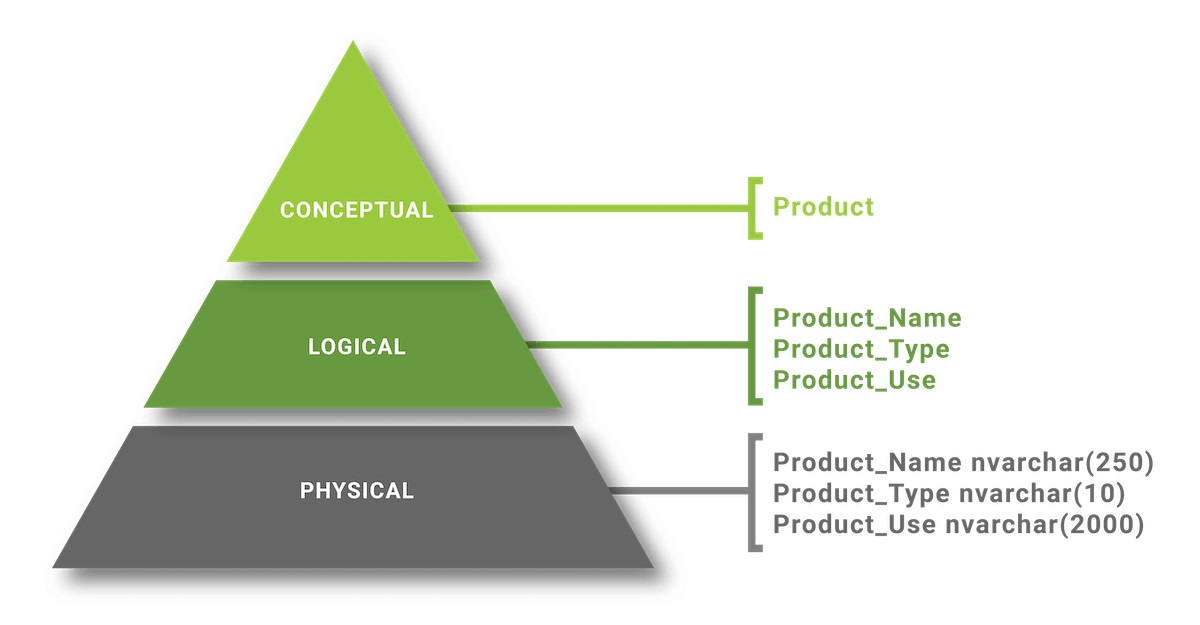
1. Conceptual Data Modeling : Data is modeled by relationships in top-tier data. The purpose of this model is to organize, scope and define concepts and rules and business processes . Once the conceptual data model is created, it can be adapted and transformed into a logical data model.
2. Logical Data Modeling : Modeled data describes data and their relationships in detail. Modeled data creates logical models of the database. The main purpose of the model is to develop a technical map of rules and data structures. The logical data model will serve as the basis for creating a physical data model.
3. Physical Data Modeling : This model describes how the system will be implemented using a particular database management system. This model is often created by data administrators and developers with the primary purpose of implementing the actual database.

Entity-Relationship Model – ER Model

Data models can be classified into 3 different groups:

• Object-based logic model
• Logical model based on records
• Physical model

Entity-Relationship (ER) models belong to the first category – object-based logic models .

The model is based on a simple idea of contacting reality. Data can be thought of as real-world objects called objects and the relationships that exist between them. For example, data about employees working for an organization can be thought of as a collection of employees and a collection of different departments (departments) that make up the organization. Both employees and departments are real-world objects. An employee of a department. Thus, a ‘belonging’ relationship associates an employee with a particular department.

An ER model contains five basic components as follows:

Entity (entity)	An entity is a real-world object that exists physically and is distinguishable from other objects. For example: personnel, departments, students, customers, accounts ….. can be called entity
Relationship (relationship)	A relationship is an association or association that exists between one or more entities. For example: belong, own, work for, save in, purchased….
Attributes (attributes)	An attribute is a feature that an entity has. Attributes help distinguish each entity from another. Example for 2 attributes student and customer, the same person but have different attributes when represented on the database: – Entity student has attributes student_id, name, age, mark. – Entity customer has attributes customer_id,name,age,phone,address
Entity set (entity set)	An entity set is a list (set) of similar objects. For example, the list of students in a school (according to a common standard with the same attributes) is called the student entity set.
Relationship set	A list (set) of relationships between two or more entity sets is called a relationship set. For example, students study many different subjects, the set of all “subject learning” relationships that exist between 2 entities student and subject can be called “learning” relationship set. subjects”

An association relationship between one or more entities and can have 3 types of relationships as follows:

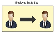
Self-relationships

The relationship between an entity and objects like it is called a self relationship . For example, a manager and a member of a team, both are personnel and belong to the same entity set. Team members work for management, so a “work for” relationship exists between 2 different HR entities but these personnel are in the same entity set.

Binary relationships

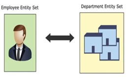
The relationship that exists between entities located in 2 different entity sets is called binary relationship . For example, an employee belongs to a department. A relationship exists between two entities located in two different entity sets. The HR entity is in the entity set (employee), the department entity is in the entity set (department).

Ternary relationship (3 person relationship)

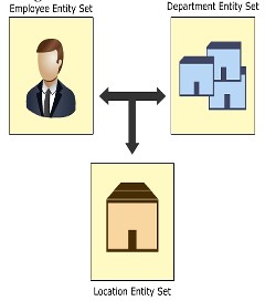
To put it simply, this relationship is a relationship of 3 participating entities, which is called a ternary relationship . For example, an employee works for the finance department in a certain branch of the organization. In here, there are 3 different entities: personnel, department, branch , and personnel will be associated with the department through the entity set representing the branch.

Relationships can also be classified according to mapping cardinalities. The different types of mapping are distinguished as follows:

One-to-one (mapping one to one)

This mapping exists when the object of one entity set can be associated with only one instance of another entity set. For example, a citizen’s citizen identification number, which will link directly and uniquely to a citizen’s motorcycle license code. It is not possible for a citizen with one identification number to have multiple motorcycle license codes. It is called a distant light or a one-to-one relationship.

One-to-many (mapping one to many)

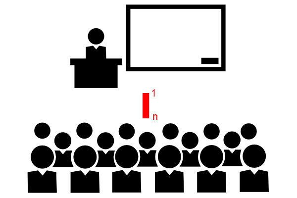
This type of mapping is used when an entity in an entity set is associated with more than one entity in another entity set. For example, if there are many students in a class, a one-to-many mapping is often used to represent this mapping. People often call it a 1-to-many relationship or a 1-to-many mapping.

Many-to-one (mapping many to one)

This type of mapping is used when multiple entities in an entity set are associated with an entity of another entity set. We understand roughly this mapping is the opposite of a one-to-many mapping. For example, a class has many students.

Many-to-many (mapping many to many)

This type of mapping is used when multiple entities of one entity set are associated with many entities of another entity set.

For example, a store has many products for sale, each customer’s order when buying will include many different products, we can see that 1 order can have many products, but one product also appears on many orders, this is the best example of a many-to-many mapping.

In addition, the ER model also adheres to some concepts as follows:

Primary key (primary key)

Primary key is an attribute used to determine the uniqueness of an entity for an entity set. In the database structure, it is usually always advisable to have a column used as the primary key in the table (entity set).

Weak entity sets

Entity sets that do not have an attribute to define a primary key are called weak entity sets.

Strong entity sets

Entity sets that have attributes to define primary keys are called strong entity sets.

Entity relationship Diagram (ER Diagram)

An ER diagram is a graphical representation of an ER model. In the ER diagram, use symbols to effectively represent the different components of the ER . model

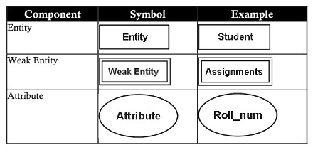
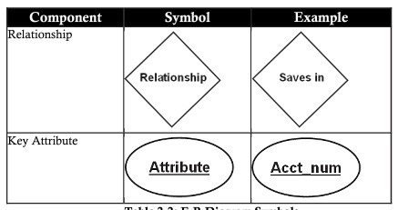
Attributes in the ER model can be classified as follows:

Multi-valued (multi-valued)

A multivalued attribute is illustrated by a two-line ellipse, which has more than one value for at least one instance of its entity. This attribute can have an upper bound and a lower bound specified for any individual entity value.

For example, the phone_number attribute can store multiple values for an entity. (A person can have more than one phone number)

Composite (synthetic)

A composite attribute itself can contain two or more attributes, the sub-attributes are basic properties and have their own independent meanings.

For example, the address attribute is usually a composite attribute, for example, when representing a company address 6/203 Truong Chinh – Thanh Xuan – HN, 6/203 Truong Chinh will be the address, Thanh Xuan will save it at District, Hanoi is City

Derived (derived attribute)

Derived properties are attributes whose value completely depends on another attribute and are represented by an ellipse composed of ellipses.

The age attribute of a person is the best example of derived attributes. For a particular person entity, a person’s age can be determined from the current date and date of birth of the person.

The steps to structure the ER diagram are as follows:

1. Collect all the data that had to be modeled.
2. Define data that can be modeled as real-world entities.
3. Identify attributes for each entity.
4. Sort entity sets into weak or strong entity sets.
5. Sort entity attributes as key attributes, multivalued attributes, composite attributes, derived attributes, etc.
6. Identify the relationships between different manipulative factors.
7. Using different symbols draw the enticement elements, their properties, and their relationships. Use proper sysbols while plotting properties.

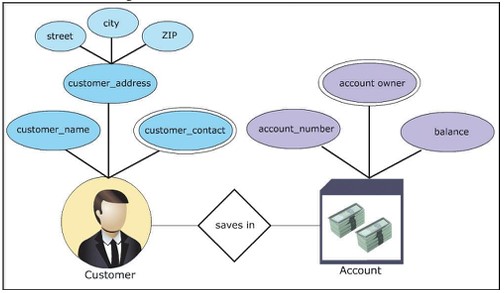
For example, building a database simulating a bank, with customer and account management. The ER diagram for the scenario can be constructed as follows:

1. Data collection: this business needs a list of accounts and customers who want to deposit money.
2. Identify entity: there are 2 entities customer, account
3. Define properties:
   1. Customer: name,address,contact
   2. Account: id,owner,balance
4. Entity Set Sorting
   1. customer: weak entity set
   2. account: strong entity set
5. Sort properties
   1. customer entity set: address – composite, contact – multi-valued
   2. accounet entity set: id – primary key, owner – multi-valued
6. Define relationship: customer deposits money in the account, the relationship will be “deposit”
7. graph Draw the ER . model

Normalization (normalization of data)

Typically, all databases are identified by a large number of columns and records. This approach has certain limitations. Consider the following example where two entities are saved in the same table of employees in projects. Include the employee’s details as well as the details of the project they are working on:

The concepts of problems encountered when data are not normalized are as follows:

Repetition anomaly

Columns like project_id, project_name, salary have data in repeated records, this repetition hinders both data retrieval performance and storage capacity. This repetition of data is called repetition anomaly

Insertion anomaly

Assume the new member of the department is a new employee named Ann. Ann is not assigned a project right now. Insert her details in the table with blank cells on columns named Project_id, Project_name. Leaving columns blank leads to some problems later on. The anomaly created by the insertion operation is called insertion anomaly.

Delete anomaly (delete anomaly/anomaly)

Assume Bob is taken from the MAGNUM project. Delete a MAGNUM project record whose employee name is Bob including employee number (employee_number), rank (grade) and salary (salary). The loss of data affects Bob’s personal information details, this loss can be seen in the table below. The data lost due to the above deletion is called deletion anomaly.

Updating anomaly

Assume John has been given a raise or a pay cut. Changes in John’s salary or grade need to be reflected in all projects that John works on. This is called updating anomaly.

---

The table detailing the employees in the department is called the unnormalized table. These limitations suggest that normalization is necessary.

Nomarlization is a process of removing unwanted redundancies and dependencies. Initially, Codd (1972) described three normalization forms (1NF, 2NF, and 3NF), all based on dependencies between the attributes of the relation. Fourth normal form (4NF) and fifth normal form (5NF) are based on multivalued and dependent association and were introduced later.

First Normal Form (1NF)

The steps to complete 1NF are as follows:

1. Create separate tables for each group of related data
2. Table columns need to store prime values (can understand primitive values)
3. All primary key attributes need to be defined

Considering the above table example, we need to normalize the table by clearly dividing the two entities project and employee

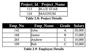
Second Normal Form (2NF)

Tables are called 2NF if the following requirements are met:

• Meet the requirements of 1NF
• there are no dependencies in the tables
• Tables are linked together through foreign keys.

Considering the example above, we use 2NF to link between the project table and the employee table (to know which employee the project is assigned to) through an intermediate table.

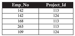
Third Normal Form (3NF)

To complete 3NF normalization, the following requirements must be satisfied:

• The table should meet the requirements of 2NF
• tables should not have dependent columns in them

Continuing the above example, in the employee table, we see that the Salary column depends on the Grade column according to the general formula: A – 20,000 | B – 15,000 | C – 10,000. So, to normalize this data, we’ll split the employee table, which stores only the grade, and a table that shows the grade and salary. When you do so, you can later add and update grades to easily meet your needs without affecting the overall data.

Denormalization

By normalizing data, redundant data is minimized. This means that the size of the required database storage space in the database will be reduced. However, they also have some limitations as follows:

• Query statements will become more complex when connecting data between different tables
• In fact, the query statement can involve more than 3 tables depending on the information needs (increasing complexity in writing query statements, y/c programmers or highly specialized DBAs)

If the join query statements are used too often, the performance of the database will decrease, the processing time of the CPU will increase, affecting the program speed. Therefore, in some cases, redundant data can still be used to increase database performance, which means accepting redundant data storage (sacrificing storage capacity to increase performance). query), called denormalization (data denormalization)

Relational Operators

The relational model is based on a solid foundation of relational algebra. Relational algebra consists of a set of operators that operate on relations. Each operator takes one or two relations as its input and creates a new relation as output. Consider the sample bank data table with the following branches:

SELECT (selection)

The SELECT operator is used to retrieve data that satisfy the required conditions. The sigmoid character (ð) is used to represent a select.

The example below is a table when selecting records with a branch in London

Or a transaction that requires taking out branches with reverses greater than 20 billion euros

PROJECT (projection)

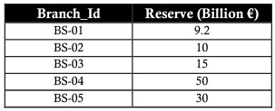
The PROJECT operator is used to refer to the details of a relational table. The PPROJECT operator displays only the required fields, and leaves out the non-required fields in the column. The PROJECT operator is represented by the pi character “π”.

The example below uses the PROJECT operator to get the id and reverse for a business without getting the branch name:

PRODUCT (multiplication/product)

The PRODUCT operator is used to superficially combine information from two related tables, represented by the character “x”.

For example, we have a loan table like this:

Use the PRODUCT operator used to combine the branch and loan tables to represent total reserves and total loans:

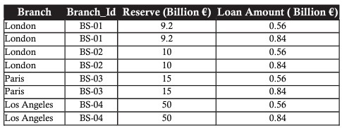
Multiplication combines each record of the first table with all the records in the second table, in other words, it creates all possible combinations between the records of the two tables.

UNION (association)

Let’s say, given the bank’s sample data above, management wants to take out branches that have reserves or loans of less than 20 billion Euros. The resulting table should contain branches with reserves or loans of less than 20 billion euros, or both columns that meet the criteria.

This visualization is the combination between two data sets, the steps in turn are as follows:

• Collection of branches with reserves of less than 20 billion Euro
• Set of branches with loans under 20 billion Euros
• Merge the 2 sets together, ensuring that the branch with the same reserves and loans under 20 billion Euros appears only once

INTERSECT (Intersection)

Suppose we want to know which of these branches has both low reserves and low lending. The solution would be to use the intersection INTERSECT operator. The INTERSECT operator produces the correct data in all the tables to which it is applied. It is based on intersection set theory and is represented by the symbol ” “ . The result will be the intersection of two tables that include the list of branches that meet both the reserve and loan criteria with less than 20 billion euros.

DIFFERENCE (Miraculous)

Going back to the above example, if we want to know which branch has low reserves but no loans, the solution is to use the (DIFFERENCE). The notation is denoted by the “-” character, its output is still a union from 2 different tables, but the difference is that it only retrieves the correct value of one table, not the other, so Branches with low reserves but no loans will not be taken out.

JOIN

Concatenation is an extension of multiplication that allows the selection of the result of the multiplication. For example, if the reserves and loans of the branches are smaller with the above PRODUCT, the data will be redundant and need to be aggregated and reduced. The output of the JOIN will return only the newly listed branches that have both reserves of less than 20 billion euros and loan capital.

DIVIDE (Dividation/quotient)

Suppose we again want to see the branch tene and the reserves of all branches that have loans. This situation needs to use the DIVIDE permission to handle. All it takes is to split the Branch Reverse Details table (2.19) by the list of branches, and the Branch_id column of the BranchLoanDetails table (2.23). The result is as shown below

Note: the properties of the division table must always be a subset of the divided table. The resulting table always leaves the split table properties blank, and the records don’t match the records in the split table.