Excel is known as a spreadsheet that is used by many people in their daily work, especially for those who work in the accounting field. When you work with Excel, it allows you to use many different types of numbers. Therefore, so that when looking at the spreadsheet, it is easy for readers to distinguish especially negative numbers from other types of numbers, you should format brackets and even highlight them in red. So how to do it, please refer to the article below.

How to close parentheses and highlight negative numbers in Excel

Normally, as we often see, in some Excel problems or in real work, many times you have to process and work with Excel spreadsheets as required to see the fastest and most accurate. Most of the time, in many documents, you need to clarify and distinguish negative numbers in your worksheet by closing brackets or, more importantly, by highlighting those cells in red. Fortunately, this feature has been very well supported by Excel, making it easy for users to quickly do it with "Custum".

Specifically, the steps are as follows:

• Step 1: First, open the text file you want to format.

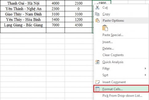
Then you highlight the column or area that you need to Format according to the requirements of closing brackets with negative numbers in the spreadsheet.

Next, you right click on the area you selected and click on “ Format Cells”.

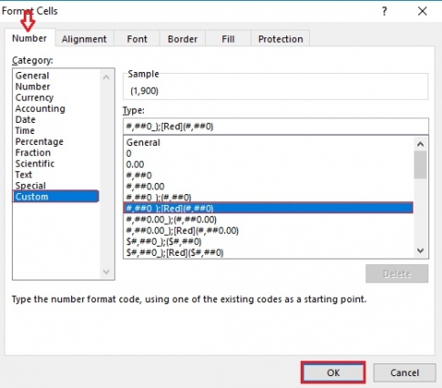
• Step 2: The Format Cells dialog box appears, select Tab Number.

In the Category table, select the "Custom" item.

Next, in the Type panel you choose the format "#,##0_);(#,##0)" as shown below and click "OK".

• Step 3: You will get results like the table below.

So instead of negative numbers with a dash in front, negative numbers have now been replaced with numbers with parentheses.

In other cases, if you still want to keep the "-" sign in front but want to highlight those numbers in red to make them easier to see and distinguish, you do the following:

• Step 1: You highlight the data area you want to format, then right-click and select "Format Cells".

• Step 2: Now the Format Cells dialog box appears.

You choose Tab Number , also in the Category section you choose "Custom".

In the Type dialog box, find the format " #,##0_);[Red](-#,##0)" then click "OK" .

After doing this, you have obtained the following results:

Note: For both ways, if in the Type section of the current version of Excel, there is no above format, we can copy and paste that format into the Type section and then click OK to apply it.

In the Format Cells dialog box there are many different formats, if you like you can do the same and explore other formats.

Conclusion: While working with Excel spreadsheets especially with data types, you need different ways to easily distinguish them. And above, I showed you two very simple ways to do it with 2 steps. If you do not know this feature, please do it, it will help you a lot in the process.

Wishing you success.