When using Excel, you work with Excel files that have too many records. At this time, viewing, comparing and contrasting data can be time consuming and error prone. The following article will help you fix the columns that need to be compared to shorten the time and bring more efficiency.

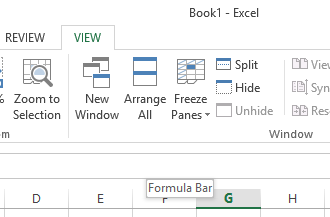
This is an article where I guide you to fix rows and columns for Excel 2013. However, if you use Excel 2007,2010,2016, the method is similar.

The article consists of 3 parts:

• Fixed row

• Fixed column

• Fixed both rows and columns.

1. Fixed row

For example, I have a data table as follows:

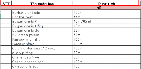
I want to freeze the row in the top red cell. Here's how to do it:

• Step 1: Locate the mouse pointer.

Place the mouse pointer in the first cell of the line below the line to be fixed. So the lines above the line where the mouse pointer is placed will be fixed.

• Step 2: You look up, select the View tab and then select Freeze Panes.

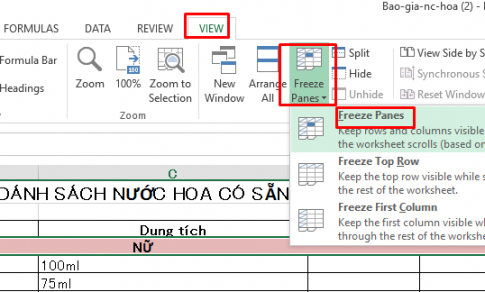
So I have fixed lines 1,2,3. Below are the results:

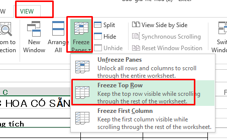
You can also freeze only the first row by going to the view tab , selecting Freeze Panes , and then choosing Freeze Top Row .

2. Fixed column

To freeze the column you do the following:

• Step 1: There are 2 ways to determine where to place the mouse pointer.

Method 1: You place the mouse at the first cell of the column after the column you want to freeze

Here to fix the column No, we place the mouse pointer in cell B3

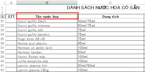
All columns before the column where the mouse pointer is placed will be fixed.

Method 2: Multiply the entire column to the right of the column you want to fix.

Here, if you want to fix the column STT, highlight the column Name perfume.

• Step 2: You look up, select the View tab , then select Freeze Panes.

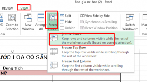
So you have fixed the STT column, let's see the results below:

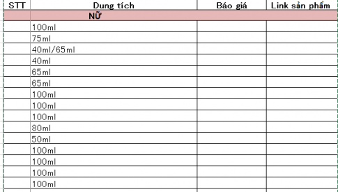
When dragging the switch bar, the column Name of perfume disappears but column STT is still displayed.

3. Fixed both rows and columns.

• Step 1: Locate the mouse pointer.

For example, you want to freeze column No and row 1,2,3-> You place the mouse pointer in cell B4.

• Step 2: You look up, select the View tab, then select Freeze Panes.

So you have the results already.

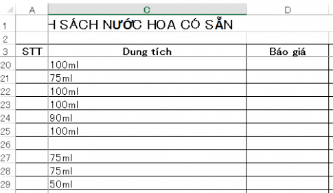
Note: To unfreeze rows and columns, you just need to go back to the View tab and select Freeze Panes . Then select Unfreeze Panes and you have unfreeze rows and columns.

Conclusion: The above article has guided you to fix rows and columns in Excel extremely simple and easy to use. When working with excel files with too much data, it is very useful to freeze columns with important data. Hope this article can be of help to you.

Good luck.