When using Excel, you use a lot of formulas in spreadsheets. However, if you don't want other people to see these recipes, you need to hide them. The following article will guide you. In this article, I hide formulas in Excel 2013. However, if you use Excel 2007, 2010, 2016, the method is similar.

Example : There is a data table as follows:

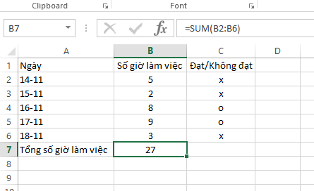
In the above example, I have a table that reports the number of hours worked each day by an employee in a working week. Finally, I calculate the total working hours of this employee using the SUM function.

So to hide this calculation formula, you just need to follow these steps:

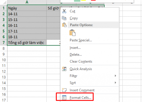
• Step 1: Highlight the above data table (Ctrl+A), right-click and select Format Cells:

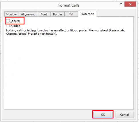
• Step 2: The Format Cells dialog box appears, go to the Protection tab, uncheck Locked and then click OK .

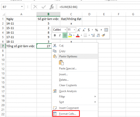
• Step 3: You select the cell with the formula you want to hide, right-click and select Format Cells:

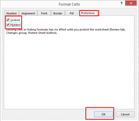
• Step 4: The Forma t Cells dialog box appears. You select the Protection tab, tick the Locked and Hidden boxes, then click OK.

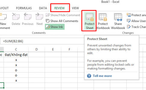
• Step 5: You select the cell to hide, look up, select the Review tab and select Protect Sheet to set a password for this formula cell.

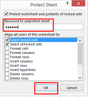
• Step 6: The Protect Sheet dialog box appears, enter the password and click OK.

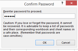
• Step 7: The Confirm Password dialog box appears, enter the password you just typed in step 6 and click OK.

So you have hidden the formula in Excel already. In this example, I have hidden the formula to calculate the total number of working hours in a week. Let's see the results:

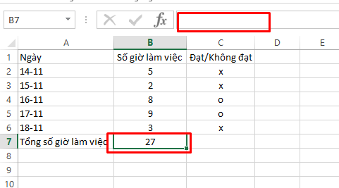
Conclusion: In this article, I have guided you to hide formulas in Excel 2013. Using Excel to calculate with functions is a familiar operation to everyone, especially those who are working in the accounting industry. Hiding this formula is extremely useful when you don't want the reader of your excel file to know how you calculated. Hope this article can be of help to you.

Good luck.