When you need to process strings in Excel, you can't help but mention the Left and Right functions. However, not everyone understands and knows how to use these two functions. Therefore, today Web888 will guide you specifically to understand more and be able to use these functions in the process of working with Excel spreadsheets.

On Excel, you will encounter many different functions such as logic functions, math functions, counting functions or string functions. In the string function, the Left and Right functions are two functions that cannot be ignored. Because its function is very good and helps you a lot in your work.

The article consists of 2 parts:

• Instructions for using the Left function in Excel
• Instructions for using the Right function in Excel

1. Instructions for using the Left function on Excel

The Left function is the function used to extract “n” characters from the Text string from the left side.

The function syntax is as follows:

Left(Text,n) or Left(Text,number_chars)

In there:

• Text : Displays a string of characters
• n : Number of characters to extract in that character string. Note: This parameter “n” may or may not be present. If not, Excel automatically defaults to 1).

Example: Given a string of characters like this: Tech12h.

Ask you to extract 4 letters from the left side so that the result is the word Tech. You just need to do the following:

=Left(“tech12h”,4) the result is Tech.

Note: For text strings, you need to enclose them in double quotes.

One more example.

We have the following data table:

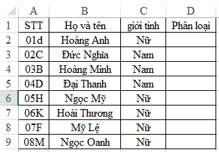
Requirements: Classify employees by getting the first two digits of the STT.

Thus, we need to separate the first 2 digits of the STT column to get the classification code.

First of all, to get the results of the sorting column, you just need to do it first with the first employee. Here, I will classify for you Hoang Anh first.

As required, we have the following calculation formula:

=Left(A2,2) the result is 01.

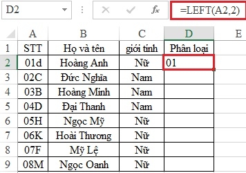
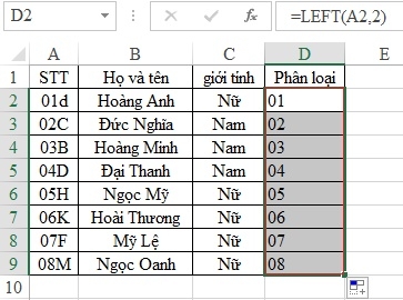
After receiving your first result, you select the result box and then move your mouse to the bottom right corner of the cell. You wait when it appears a big plus sign, then hold down the mouse and drag it to the cell where you need to perform the calculation. After releasing the mouse, you will get the results you want.

2. Instructions for using the Right function in Excel

The Right function is also a string handler like the Left function. The only difference is that instead of the Left function extracting characters from the left, the Right function extracts characters from the right side.

Specifically, the Right function is as follows:

The Right function is the function used to extract “n” characters from the Text string from the right side.

The function syntax is as follows:

=Right(Text,n) or Right(text,number_chars)

In there:

• Text: Represents a string of characters
• n : Number of characters to extract from the string. Note: This parameter may or may not be present. If there are no parameters, Excel defaults to 1.

Example: You have a string like this: tech12h.com

Ask you to extract 3 characters from the right side.

You proceed as follows:

=Right(A2,2) the result is com .

Or another example.

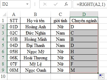
We have a data table:

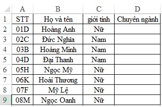
Requires you to separate 1 character from the right side of the column STT to make the name of the major.

Then we have the following formula:

=Right(A2,1) we get the result of your specialization Hoang Anh is “ D ”. Then, to do with the rest, you just need to wait for the big plus sign to appear in the lower right corner of the cell, then hold the mouse and drag to the position you need to release the mouse to get the results immediately.

So, with what I have instructed above, I hope you can understand and use the two functions Left and Right in a simple way. With Excel, you still have a lot of functions to use, if interested, you can refer to the article about Excel functions to know more.

If you find this article useful, you can share it to let more people know. Thank you!.