With reports that have many related data to compare, the easiest way to show it to others is in the form of a chart. However, have you understood the operations to draw charts in Excel yet?

The following article will detail how to draw the simplest charts on Microsoft Excel 2013 version, and basically they can be manipulated on all other versions.

1. Create a chart

To create a chart in Excel, you start by entering numerical data for the tables on a worksheet. You can then plot that data into a chart by selecting the type of chart you want to use on the Office Fluent Ribbon.

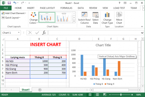
• Create the table data you want to convert to the chart, go to Insert and select the Chart group

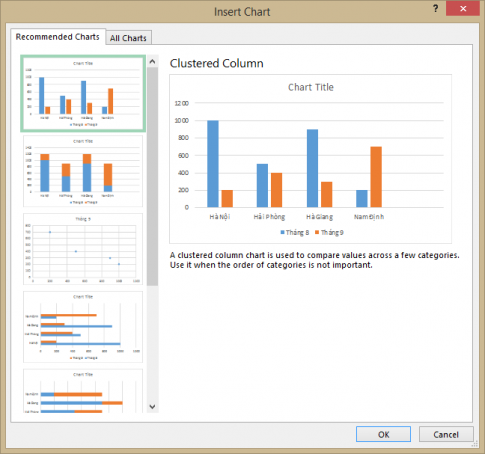
The Insert chart window appears, allowing you to choose the appropriate chart type. After selecting the chart, select OK to finish.

• Result:

2. Edit chart

• Title

To insert the Title of the Graph, in the Chart Tools you choose Layout -> Chart Title and select the display style

– Centered Overlay Title : The title of the Graph will be displayed on top and does not allow changing the size of the graph.

– Above Char t: The title of the graph will be displayed above the graph area and the size of the graph can be changed.

• Axes

When working with the unit chart dividing on the vertical axis will take the default value. To change the division value on the vertical axis, do the following:

– Right click on the value column on the vertical axis, select Format Axis

The Format Axis window appears, choose the size you need in the Major Unit section.

– Minimum: Determines the minimum value on the axis (start value)

– Maximum: Specifies the maximum value on the axis (end value)

• Customize captions, titles

– Depending on the type of chart being processed, Excel allows you to edit the title types of that chart type.

– To add titles for the horizontal (or vertical) axis go to Chart Tools–> Layout –> Labels –> Axis Titles –> and select the appropriate style.

• Move chart:

– Left click and hold, drag and drop at the position you want.

• Change the size:

At the button where the map appears, you can adjust the size accordingly.

• Copy chart

– We use Ctrl + C then Ctrl + V as usual

• Clear chart

– Select the graph then press the Delete key to delete the graph. To delete a Chart Sheet , first select Chart Sheet , then right-click and select Delete from the context menu

• Print chart

– Printing the chart is like printing other Excel objects, before printing we should choose Print Preview to make sure the page prints all the content.

– If you want to print the graph as a separate page, select the graph and click the Print button to print, then Excel indicates the command to print the graph you are choosing.

Good luck!