When you have to work with too much data in Excel, to avoid mistakes, you need to distinguish those data. Excel supports you how to color cells according to the desired value. In this article, I will guide you to change the color of the cell according to a simple and fastest value.

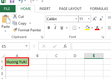
Here, I show you how to change the color of the cell according to the value applied to Excel 2013. However, if you use Excel 2007, 2010, 2016, the method is similar.

To change the color of a cell by value in Excel 2013, simply follow these steps:

• Step 1: You go to Excel, look up, select the "Home" tab then select "Conditional Formating" and select "Manage Rules…"

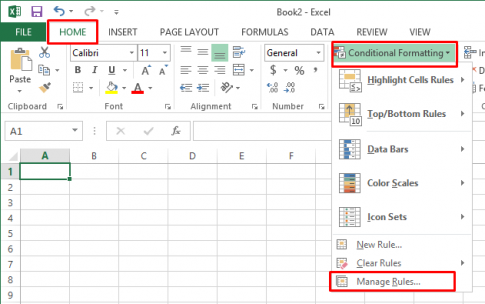
• Step 2: The rule management window appears. Click the “New rule” button to create a new rule.

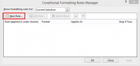
The “Select a Rule Type” section has the following options:

+Format all cells based on their values : Format all cells.

+Format only cells that contain: Formats a cell according to its value.

+Format only top or bottom ranked values: Format the top and bottom cells according to rank.

+Format only values that are above or below average: Format cells with values above or below average.

+Format only unique or duplicate values: Format cells with unique or duplicate values.

Use a formula to determine which cells to format: Use a formula to indicate which cells are formatted.

Example: Here, you want to color a cell according to its value. You will select “ Format only cells that contain ”. In the "Edit the Rule Description" box :

At "Format only cells with" the first cell you choose "Cell value" ie based on the value of the cell.

The next cell you choose " equal to " means the value in the cell must be equal to the value you want to enter in the 3rd cell. (I call this cell the value A)

Here I will choose as shown below:

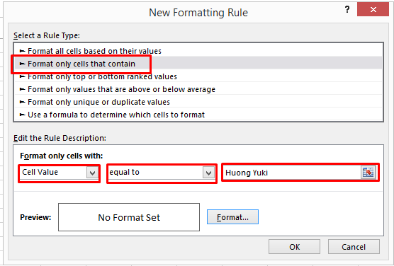
So, my A value will be “Huong Yuki”.

• Step 3: After you have selected the condition, select “Format”. When clicking Format, the screen will display as follows:

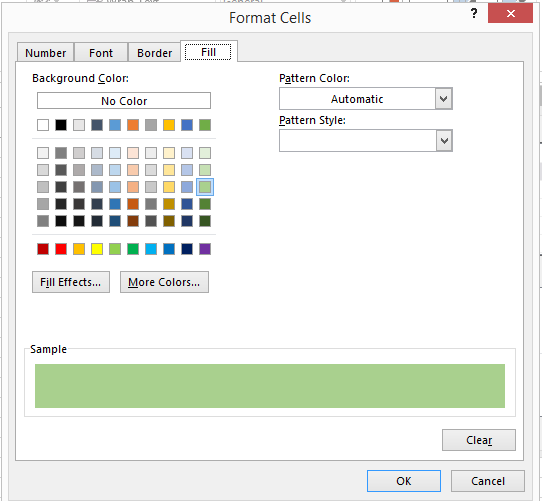
Here you choose the color for the cell and click the ok button

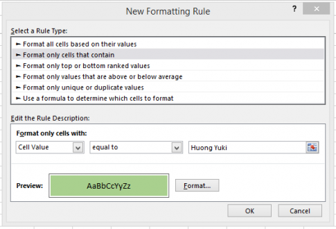
I choose the blue color as above, click OK. So you have finished adding the rule.

• Step 4: You choose a value for “Applies to” to determine which cell, column, or row this rule will apply to. For example, I choose as shown below and click Ok.

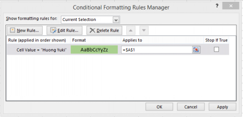
• Step 5: You enter the value A (here my A value is Huong Yuki) in cell A1 and let's see the results:

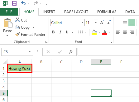
Note: Only when you enter the desired value previously entered in the correct “Applies to” box will the background color be changed.

Conclusion: In this article, I have shared with you the trick to change the color of cells by value in Excel 2013. When there is too much data to manage, changing this color is extremely useful. Hope this article can be of help to you.

Good luck.