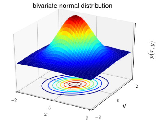
The normal distribution is also known as the Gaussian (bell-shaped) distribution. The distribution has the same general form, only the position parameter (mean μ) and the ratio (variance σ ² ) are different.

The Gaussian distribution has the form:

In there:

• Mean vector (expected): μ ∈ R ^d
• Covariance matrix : ∈ R ^dxd

For classification problems, x is known to be continuous random (when x is continuous, its possible values fill an interval on the number line X ∈ (x _min ; x _max ). We can use the Gaussian Discriminant Analysis (GDA) model: predict the probability P(x|y) based on a normal distribution of many variables.

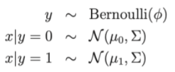
Write as a distribution:

In there:

• Model parameters , , μ ₀ , μ ₁ .
• μ ₀ , μ ₁ are the two average vectors of x|y = 0 and x|y = 1
• The loss function of the model: Log-linkihood

Thus, to pole at the loss function, we can reduce the problem to finding the parameters , , μ ₀ , μ ₁ of the training dataset.

Let's discuss some issues between GDA and Logistic regression.

Suppose if we consider p(y=1 | ∅, Σ , μ ₀ , μ ₁ ) is a function of x, then the expression will now have the form:

Where theta is an approximation of , , μ ₀ , μ ₁

Thus we see that it has the same form as the logistic regression algorithm.

• So if the distribution of p(x | y) has a Gaussian distribution, then the GDA is good
• If the distribution of p(x | y) is not Gaussian, then GDA may be less efficient.

Naive Bayes classification algorithm

Suppose an algorithm classifies customers or classifies emails as spam or non-spam. If we represent email as a feature vector with dimensions equal to the size of the dictionary. If in the email there is the jth word in the dictionary then x _j = 1 otherwise x _j = 0. And what if the set of word points consists of 5000 words, x ∈ {0, 1} ⁵⁰⁰⁰ . So, if you want to build a classifier, you need at least 2 ^(50000-1) parameters and that's not a small number.

To model p(x | y) we assume that xi is independent. This assumption is called Naive Bayes (naive). The result of the algorithm is Naive Bayes classifier.

The probability p(c | x) is calculated by:

To calculate p(x|c), we rely on the assumption that xi is independent of

The larger d is, the smaller the probability of ohari is. So we need to get the log on the right side to scale it up.

Distributions commonly used in NBC.

1. Guassian naive Bayes:

For each data dimension i and a class c, xi follows a normal distribution with expected μ _ci and variance σ _ci ² .

The parameter μ _ci and the variance σ _ci ² are determined based on the points in the traning set of class c.

2. Bernoulli Naive Bayes

The components of the feature vector are discrete variables that take the value 0 or 1: Then p(xi|c) is calculated by:

p(i|c) can be understood as the probability that word i appears in the text of class c.

3. Multinomial Naive Bayes:

The components of the feature vector are discrete variables according to the Poisson distribution.

Assume a text classification problem where x is a Bow representation.

The value of the ith element in each vector is the number of times the ith word occurs in the text.

Then, p(xi|c) is proportional to the frequency with which word i appears in documents of class c.

N _ci is the total number of times i appear in the documents of class c.

Nc is the total number of words (including repetition) appearing in class c.

4. Laplace smoothing.

If there is a word that never appears in class c, then the probability of going to the right of the following formula will be = 0.

To solve this, a technique called Laplace smoothing is applied:

Where α is a positive number, usually α will equal 1, the sample plus dα helps to ensure the total probability. Thus, each class c will be described by a subset of positive numbers that sum to 1.