While we use the available libraries to train the model, but we use a locking spoon to open a box without knowing what is inside it? But you can still open the box. With a better understanding of the theories inside the algorithm, you can use the parameters to fit the model.

In this section, I will familiarize you with linear regression which is one of the most basic algorithms in machine learning. In this algorithm, the input and output are described by a linear function.

Illustrated math problem

Suppose there is a problem of predicting house prices. There is data of 1000 houses in that city, in which we know the parameters in the word house is the width is x ₁ m ^₂ has x ₂ bedrooms and is ₃ km from the center. If you add a new house with the above parameters, you can predict the price y of the house? If yes, what form does the predictor function y = f(x) look like? Here feature vector x = [x _1, x ₂ , x ₃ ] ^_T is a column vector containing input information, the output y is a scalar.

In fact, we can see that as the coefficients of the word features increase, the output also increases so there is a simple linear function:

y_pre = f(x) = w ₀ + w ₁ x ₁ + w ₂ x ₂ + … + w _n x _n = x ^_T w

In there:

• y_pre: is the predicted output value. (and y_pre will be different from actual y)
• n is the number of features.
• (x _i ) is the i .th feature
• w is the parameter of the model where w ₀ is the bias and the parameters w ₁ , w ₂ ,….

The above problem is the problem of predicting the value of the output based on the input feature vector. In addition, the value of the output can take on many different positive real values. So this is a regression problem. The relationship y_pre = x ^T w is a linear relationship. The name linear regression comes from here.

Model training

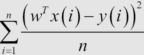
After having a linear regression model, the training of the model is about finding the most optimal parameters through the training data set. To do this we need a way to determine if the model is good or not. Here I will introduce a way to determine that is to use the expression Root Mean Square Error (RMSE). The goal of that training is to minimize the value of Mean Square Error (MSE). It simply means that we want the difference between the predicted y and the actual y to be as small as possible.

Average 1/n, or sum in the loss function, mathematically does not affect the solution of the problem. In machine leanring, the loss functions usually contain the average coefficient for each data point in the training set, so when calculating the value of the loss function on the test set, we need to calculate the average error of each point. Calculating the loss function helps to avoid overfitting when the number of data points is too large and it also helps us to evaluate the model later.

Standard Equation

To find the value of w that helps the above equation to reach its minimum value, we can calculate the derivative of the upper direction with respect to w when they are zero. And determine the minimum.

Therefore, we can determine the minimum by the following formula: w = (X ^T X) ^– 1XTy.

Where w is the value at which MSE(w) is minimized. y is the vector to find including (y ¹ , … y ^m ).

Implement in python.

Assuming the data set below, determine the weight of that person by height.

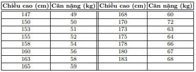
Data display

import numpy as np
import matplotlib.pyplot as plt

X = np.array([[147, 150, 153, 158, 163, 165, 168, 170, 173, 175, 178, 180, 183]]).T

y = np.array([ 49, 50, 51, 54, 58, 59, 60, 62, 63, 64, 66, 67, 68])

Looking at the problem, we need to determine the model of the form: (weight) = w_1*(height) + w_0.

Determine the solution according to the formula.

Initialize data

one = np.ones((X.shape[0], 1)) #Bias
Xbar = np.concatenate((one, X), axis = 1) # each point is one row

Next, we will calculate the coefficients w_1 and w_0 based on the formula . Note: the pseudo-inverse of a matrix A in Python will be calculated using numpy.linalg.pinv(A ).

A = np.dot(Xbar.T, Xbar)
b = np.dot(Xbar.T, y)
w_best = np.dot(np.linalg.pinv(A), b)

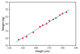
Use the model to predict the data in the test set:

y1 = w_1 * 155 + w_0

y2 = w_1 * 160 + w_0
print('Input 155cm, true output 52kg, predicted output %.2fkg' %(y1) )
print('Input 160cm, true output 56kg, predicted output %.2fkg' %(y2))

Result

Input 155cm, true output 52kg, predicted output 52.94kg
Input 160cm, true output 56kg, predicted output 55.74kg

You can also try with some python libraries to compare the results.

Problems that can be solved by linear regression

We see that the formula X ^T W is a linear function of both w and x. But in fact linear regression can be applied to models that only need to be linear with respect to w. For example:

y w ₁ x ₁ + w ₂ x ₂ + w ₃ x ² ₁ + w ₄ sin(x ₂ ) + w ₅ x ₁ x ₂ + w ₀

Is a linear function of w and can therefore also be solved by linear regression. However, determining sin(x2) and x1x2 is relatively unnatural.

Limitations of linear regression

The first limitation of linear regression is that it is very sensitive to noise. In the height-weight relationship example above, if there is only one noisy data pair (150 cm, 90 kg) the results will be very different.

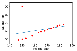
So before implementing the training model we need a step called pre-processing that I talked about in the previous blog you can refer to.

The second limitation of linear regression is that it cannot represent complex models.

summary

So in this article, I showed you how to train a linear regression algorithm. Basically, to train an algorithm it takes:

• Define the model.
• Define a cost function (or loss function).
• Optimizing the cost function using training data.
• Find the model weights where the cost function has the smallest value.